D2.2 Determine and compare the theoretical and experimental probabilities of an event happening.
Activity 1: Theoretical Probability
The following instructional scenario illustrates how teachers can lead students to develop a better understanding of the concepts related to theoretical probability and, in the process, develop more in-depth probabilistic thinking. This activity also highlights a mistake that many people make when it comes to probability, which is to not consider all possible outcomes.
The Two-Coloured Tokens Game
The teacher groups the students into teams of three. The teacher gives each team two two-coloured tokens (for example, one green side and one red side). The teacher then presents the following situation to the students:
Three students decide to play a game of tossing two two-coloured tokens into the air. They agree beforehand that Student A wins if the outcome of the tosses is two green sides (  ) , Student B wins if the outcome is two red sides (
  ) and Student C wins if the outcome is two different colours (
  ). Do you think this game is fair?
A game is fair if the probability of winning for each person is the same.
Step 1: Taking a Stand
The teacher first asks each student to tell the other members of their team whether or not they think the game is fair, without giving a reason.
Note: Asking students to take a position early in the activity builds interest and engagement, as they will then tend to want to show that they are right, and if they are not, they will want to understand why. In addition, since students are likely to base their response on an intuitive understanding of probability, teachers will be able to get a good sense of their level of probabilistic thinking and will be able to assess the presence of misconceptions about probability.
The teacher then asks each student to justify their choice to the members of their team. Student A, for example, might argue that the game is fair since each student has been assigned one of the three possible outcomes of throwing the two two-coloured tokens, in other words, RR, RG, and GG. Students should discuss the arguments presented among themselves and try to agree on a common position for the team. Some students may find that what they perceive as obvious may be perceived differently by others. This questioning goes a long way to changing some of the misconceptions in probability.
Step 2: The Experiment
The teacher then suggests that the students conduct an experiment to see if the team's choice seems correct. Each team must throw the two tokens 10 times, record the results, and analyze them to see if the results confirm or contradict their position.
Teachers prepare a results table and ask each team to record their data in it.
Here is an example of possible outcomes:
Results of the Two-Coloured Tokens Throws
| Team | Red, Red | Green, Green | Red, Green |
|---|---|---|---|
| Team 1 | 3 | 3 | 4 |
| Team 2 | 5 | 0 | 5 |
| Team 3 | 2 | 2 | 6 |
| Team 4 | 3 | 2 | 5 |
| Team 5 | 1 | 3 | 6 |
| Team 6 | 3 | 4 | 3 |
| Team 7 | 2 | 0 | 8 |
| Team 8 | 1 | 2 | 7 |
| Team 9 | 5 | 2 | 3 |
| Team 10 | 2 | 4 | 4 |
Teachers lead a discussion about the results presented in the table by asking students questions such as:
- Have any teams changed their initial choice of whether or not the game is fair after looking at the results? If so, why?
Note: Given the small number of trials, it is quite possible that one team's position is the correct one, but that the results of the experiment suggest otherwise.
- What do you see when you compare the results of the different teams? (There is a lot of variability in the results.)
- Based on the results, which teams might conclude that the game is fair? That it is not fair?
The teacher then discusses with the students how difficult it is for each team to draw conclusions after only 10 trials. To increase the reliability of the conclusions, they suggest that the class consider all the results from all the teams. Summing the results in each column yields the following table.
Results of the Two-Coloured Tokens Throws
| Red, Red | Green, Green | Red, Green | |
|---|---|---|---|
| Total of 100 throws | 27 | 22 | 51 |
Teachers encourage students to analyze this data by asking questions such as:
- What do you see about the number of R R and G G results? (The number of R R results is very similar to the number of G G results.)
- What do you see about the number of R G results? (It is significantly higher than the number of R R results and the number of G G results. In fact, it is almost equal to the sum of the R R and G G results.)
- What do these data seem to indicate about the game? Why? (The data seem to indicate that the game is not fair, because Student C seems to have a higher probability of winning than the other two students.)
- If 100 more trials were done, is it possible that the data would lead us to believe that the game is fair? (If we take into account the variability of the results that each team has achieved, this is indeed possible.)
Step 3: Theory
The teacher points out to the students that it would be important to find another way to determine if the game is fair or not. The teacher suggests that the students analyze more carefully the possible outcomes of throwing two two-coloured tokens. To facilitate this analysis, the teacher writes the number 1 on both sides of the first token and the number 2 on both sides of the second token. The teacher then explains to the students that if the first token is thrown, there are two possible outcomes, either a green side or a red side, and that these two outcomes are equally likely. Then, following the achievement of each of these two results, one can also obtain a green side or a red side by launching the second token. The results of the two tokens' tosses can be represented using the following tree diagram or table.
image Tree diagram. First chip: green; second chip: one green chip, one red chip. First chip: red; second chip: one green chip, one red chip. Tableau : The first row of the table is named "First Green Chip" and the second row is named "First Red Chip". The first column is named "Second green chip" and the second column is named "Second red chip". In the box corresponding to the first green chip and the second green chip, there are two green chips. In the box corresponding to the first green chip and the second red chip, there is one green chip and one red chip. In the box corresponding to the first red chip and the second green chip, there is a red chip and a green chip. And in the box corresponding to the first red chip and the second red chip, there are two red chips.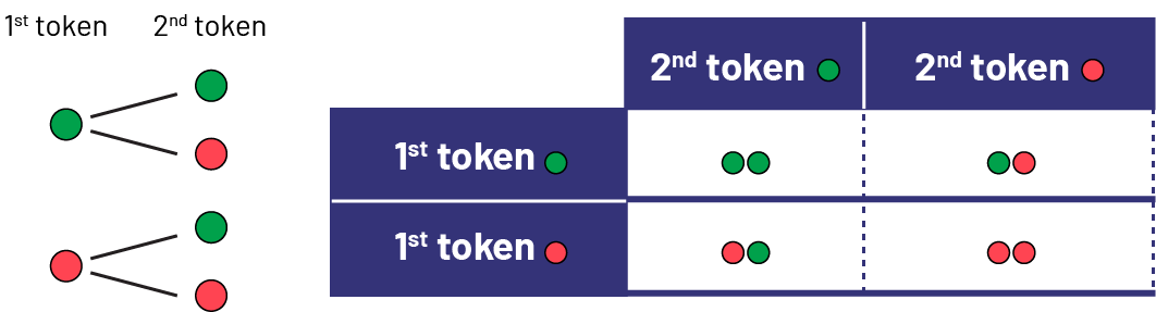
Looking at these results, we see that there is one way to get two green tokens, one way to get two red tokens, and two ways to get two differently-coloured tokens. The probability of getting two tokens of different colours is therefore greater than that of getting two red tokens or of getting two green tokens, which confirms that the proposed game is not fair.
We can also observe that there are two ways to get two different coloured tokens (G R and R G) and two ways to get two tokens of the same colour (R R and G G). The probability of getting two different colours (red and green or green and red) is therefore equal to the probability of getting the same colour, either two reds or two greens. The results of the 100 trials shown in the table above illustrate these probabilities quite well (51 R G or G R results and 49 R R or G G results).
Teachers can also ask students if the conclusions would be different in a situation where the same two-coloured token is thrown twice. The goal is to have students recognize that the two situations are the same, since they are independent outcomes, in other words, the outcome of the second token throw does not depend on the outcome of the first token throw. Therefore, there is no difference in the possibilities between two successive throws of a single token or a single throw of two tokens.
Note: Many students have difficulty accepting that their initial take is not correct, even when a theoretical explanation is provided. To help them, it is important to expose them to a variety of probability experiments.
Source: translated from Guide d’enseignement efficace des mathématiques, de la 4e à la 6e année, Traitement des données et probabilité, p. 151-155.
Activity 2: A Remarkable Spinner (Comparison of Experimental and Theoretical Probability)
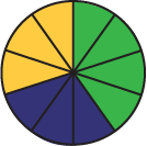
Group students into ten teams. Give each team a paperclip and a copy of Appendix 6.5A, Appendix 6.5B and Appendix 6.5C. Ask students to colour or label one fourth of the circle on Appendix 6.5A yellow, one fourth blue and one half green.

Have them put the paperclip in the center of the circle, spin it 10 times, record the results, and represent them by colouring or labelling the appropriate sections of the circle in Appendix 6.5B.
Example
By spinning the paperclip 10 times, it stopped four times in the green section, three times in the blue section and three times in the yellow section.
Invite teams to post their results on the board.
Example
image Ten pie charts divided into ten equal parts are placed in two rows of five. They each represent a team. Team One's pie chart has 8 green and two yellow parts. Team Two's diagram has five navy blue parts, two green parts and three yellow parts. Team Three's diagram has seven green parts and three navy blue parts. Team Four's diagram has four green parts, four yellow parts and two navy blue parts. Team Five's diagram has six green parts, two yellow parts and two navy blue parts. Team Six's chart has four green parts, two yellow parts and four navy blue parts. Team Seven's chart has five green parts, two navy blue parts and three yellow parts. Team eight's diagram has six green parts, three navy blue parts and one yellow part. Team nine's diagram has six green parts, two navy blue parts and two yellow parts. And the diagram for team ten has six green parts, one navy blue part and three yellow parts.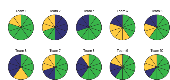
Facilitate a discussion to highlight the variability in results, asking students questions such as:
- What do the spinners on the board represent?
- What can you say about these representations?
- Why didn't you all get the same results?
- Using these representations, could you easily make a connection to the distribution of colours on the initial spinner? How?
With the students, group all the data from each team into a table and determine the sum of the frequencies of the results for each colour. Then project these sums on an overhead of Appendix 6.5 C.
| Team | Green | Blue | Yellow |
|---|---|---|---|
| 1 | 8 | 0 | 2 |
| 2 | 2 | 5 | 3 |
| 3 | 7 | 3 | 0 |
| 4 | 4 | 2 | 4 |
| 5 | 6 | 2 | 2 |
| 6 | 4 | 4 | 2 |
| 7 | 5 | 2 | 3 |
| 8 | 6 | 3 | 1 |
| 9 | 6 | 2 | 2 |
| 10 | 6 | 1 | 3 |
| Total | 54 | 24 | 22 |
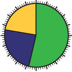
Encourage students to compare the coloured areas in Appendices 6.5A and 6.5C, and relate the number of trials, the frequency of each outcome, and the theoretical probability.
Example
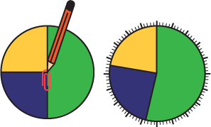 image Two pie charts are placed side by side. The first one is divided into three parts: a green part, which is half, a yellow part and a navy blue part, which are each a quarter. In the middle of the circle, there is a red paperclip and a wooden pencil that has its tip touching the center. The second one is divided into three parts. The green part takes 54 percent of the space. The navy blue part takes 24 percent of the space. And the yellow part takes 22 percent of the space.
Source: translated from Guide d’enseignement efficace des mathématiques, de la 4e à la 6e année, Traitement des données et probabilité, p. 238-240.
Activity 3: What is Your Spinner? (Theoretical Probability)
Group students into teams. Provide each team with a copy of Appendix 6.6 - Spinner Templates, a paperclip and a set of theoretical probabilities (see examples below).
Note: Use only fractions whose denominator is a divisor of 12 and ensure that the sum of the probabilities is equal to 1.
Examples of Theoretical Probability Sets
\(P(red)=\frac{1}{3},\ P(blue)=\frac{1}{2},\ P(green)=\frac{1}{6}\)
\(P(red)=\frac{1}{2},\ P(blue)=\frac{1}{6},\ P(green)=\frac{1}{3}\)
\(P(red)=\frac{2}{3},\ P(blue)=\frac{1}{4},\ P(green)=\frac{1}{12}\)
\(P(red)=\frac{1}{12},\ P(blue)=\frac{2}{3},\ P(green)=\frac{1}{4}\)
\(P(red)=\frac{1}{4},\ P(green)=\frac{3}{4}\)
\(P(red)=\frac{1}{3},\ P(blue)=\frac{1}{3},\ P(green)=\frac{1}{3}\)
Ask students to colour Spinner 1 so that it represents their assigned set of theoretical probabilities. When the teams have finished, group the teams into pairs, telling them not to show their spinner to the other team. Explain to them that the game consists of trying to determine, in turn, the theoretical probabilities represented on Spinner 1 of the other team. To do this, team A hides their Spinner 1, spins the paperclip in its center and informs team B of the colour of the sector where the paperclip stops. Team B records this result and asks Team A to spin the paperclip again. When Team B thinks they have a good idea of the colour distribution on Team A's Spinner 1, they represent this distribution on their copy of Spinner 2.
image On a surface, three objects are placed side by side: a white sheet of paper on which a wooden pencil begins to write, a card that stands upright, and a pie chart divided into twelve parts: five green parts, three navy blue parts, and four red parts. In the middle of the chart, there is a red paperclip and a wooden pencil that has its tip touching the center.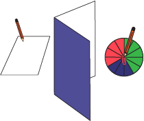
Both teams then switch roles and resume the game, this time Team A notes on their copy of Spinner 2 what they believe to be a good distribution of colours from Team B's Spinner 1. When both teams have played, students compare the spinners to determine which team was most successful in representing the opposing team's spinner.
Source: translated from Guide d’enseignement efficace des mathématiques, de la 4e à la 6e année, Traitement des données et probabilité, p. 241-242.