D1.5 Determine the range as a measure of spread and the measures of central tendency for various data sets, and use this information to compare two or more data sets.
Skill: Determining the Range and Measures of Central Tendency to Compare Sets of Data
Statistical measures are numbers used to describe a set of data. For example, the mean is a statistical measure. Statistical measures are presented as part of the fourth step in the inquiry process, interpreting the results, because they are another way of attributing meaning to the data and can provide information on which to base a decision.
Various statistical measures are commonly used in data management. Those studied in the Junior Division are range, mode, median, and mean. Students need to understand what each represents in order to select, determine, and use them appropriately.
Source: translated from Guide d’enseignement efficace des mathématiques, de la 4e à la 6e année, Traitement des données et probabilité, p. 107.
Students will then be able to use the information from the statistical measures to be able to compare sets of data.
Knowledge: Range of Data
When we look at a set of quantitative data, we often look for the maximum and minimum values of the data. These extreme values define, in our minds, the interval within which all the data lie. In data management, however, we are also interested in the size of this interval. This size is called the range of the data set. The range is the number that corresponds to the difference between the maximum and minimum values of the data.
The range gives a measure of the variability of the data. If the range is small, we know that there is little variability because the data is grouped within a small interval. If the range is large, there is a lot of variability because the data is spread over a larger interval.
Example
Here is the data for the maximum daily temperature, in degrees Celsius, for a city during the months of July and August.
| Maximum Temperatures in July (°C) | ||||||
|---|---|---|---|---|---|---|
| 32 | 33 | 33 | 34 | 31 | 25 | 25 |
| 24 | 26 | 26 | 28 | 29 | 28 | 27 |
| 30 | 32 | 33 | 31 | 29 | 29 | 26 |
| 27 | 28 | 30 | 31 | 28 | 27 | 29 |
| 30 | 30 | 25 | ||||
| Maximum Temperatures in August (°C) | ||||||
|---|---|---|---|---|---|---|
| 17 | 20 | 19 | 25 | 27 | 28 | 30 |
| 29 | 27 | 22 | 21 | 20 | 25 | 29 |
| 32 | 33 | 33 | 27 | 24 | 17 | 21 |
| 26 | 25 | 27 | 24 | 21 | 23 | 25 |
| 16 | 18 | 19 | ||||
In the month of July, we see that the lowest temperature is 24°C and the highest temperature is 34°C. The range of this data is therefore 10°C (34 – 24). In the month of August, we see that the range of the data is 17°C (33 – 16). We can therefore conclude that the maximum daily temperature in this city varied more in the month of August than it did in the month of July. This kind of information could be useful, for example, in determining the month in which one prefers to take a vacation.
Note: It is obviously not possible to determine the range of qualitative data (for example, students' favourite foods as represented by the graph below) since we cannot set a maximum or minimum value for such data.
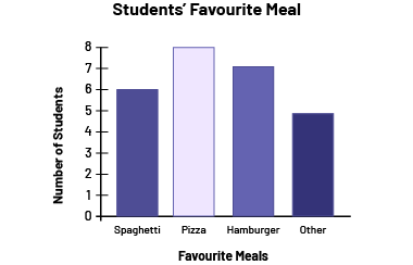 image The four bar graph with varying shades of purple is titled "Students' Favorite Meal". The horizontal axis is named "Favorite Meals" while the vertical axis is named "Number of Students." The first bar, "Spaghetti," reaches the number 6. The second bar, "Pizza," reaches the number 8. The third bar, "Hamburger," reaches 7. And the fourth bar, "Other," reaches the number 5.
Source: translated from Guide d’enseignement efficace des mathématiques, de la 4e à la 6e année, Traitement des données et probabilité, p. 107-108.
Knowledge: Measures of Central Tendency (Mode, Mean, Median)
Mode
The mode of a set of data represents the data item with the greatest frequency, that is, the data item(s) that appear most often. The mode is particularly significant in survey settings where is it necessary to determine what is the most popular, most sold, most frequent, etc. As the examples below illustrate, it is possible to determine the mode of a quantitative or qualitative set of data.
Example 1
The table below shows the data corresponding to the number of children in the families of the students in the class. It can be seen that the most frequent number is 2, indicating that there are more families with two children. The mode of this quantitative set of data is therefore two children per family.
Number of Children in the Families of the Students in the Class
| Number of Children in the Family | Number of Students |
|---|---|
| 1 | 3 |
| 2 | 12 |
| 3 | 6 |
| 4 | 3 |
| more than 4 | 2 |
Example 2
The following graph looks at the preferred colours of the students in the class. To determine the mode of this qualitative data, we need only look at the length of the bars. We see that the red and blue bars are of equal length and are longer than all the others. In this case, there are two modes, red and blue.
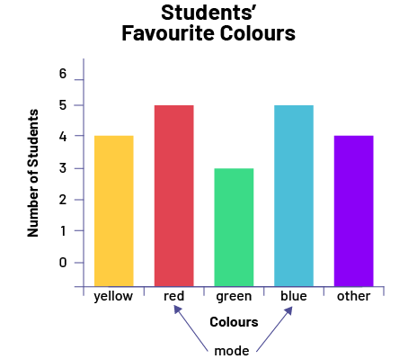 image The coloured five bar graph is titled: "Students’ Favorite Colours". The horizontal axis is named "Colours", while the vertical axis is named "Number of Students". The yellow bar goes up to the number 4. The red bar goes up to number 5. The green bar goes up to the number 3. The blue bar rises to the number 5, and the purple bar meaning "Other" rises to the number 4. With arrows, the word "mode" points to the red bar and the blue bar.
Example 3
The data below was recorded during a long jump competition.
- 1.04 m; 1.06 m; 1.12 m; 1.13 m; 1.16 m; 1.19 m; 1.22 m; 1.28 m; 1.36 m
Since all the values are different, we cannot speak of one value having the highest frequency. Therefore, this data set has no mode. On the other hand, we could choose to group the data into categories as in the table below. In such a case, the mode corresponds to the category with the highest frequency, namely the category from 1.10 m to 1.19 m.
Long jumps
| Length (m) | Number of Students |
|---|---|
| 1.00 to 1.09 | 2 |
| 1.10 to 1.19 | 4 |
| 1.20 to 1.29 | 2 |
| 1.30 to 1.39 | 1 |
When using the mode to answer a question of interest or to make a decision, it is important to consider the entire set of data. In some situations, the most frequent data item may not necessarily make the best sense of the data. It is important to encourage students to examine each situation closely before making conclusions based on the mode.
Examples of situations in which the mode is an appropriate measure of central tendency to use as a representative of the data include:
- In example 1 above, the mode of two children per family seems fairly representative of the situation, since there is a significant difference between this frequency and the others.
- In example 2 above, not only are there two modes (red and blue), but the difference between their frequency and the other frequencies is not very large. Therefore, it is difficult to conclude that these two modes represent a strong colour preference. In this case, it would be better to mention that red and blue are slightly more popular, but that yellow follows closely behind.
- In the stem-and-leaf plot below, the mode corresponds to 72 heartbeats per minute. It can be seen that this number is also part of the interval (70 to 79) that has the most data. Therefore, we can conclude that it represents this data set well.
| Number of Heartbeats per Minute of Students in the Class | |
|---|---|
| 6 | 3 5 5 8 9 |
| 7 | 1 1 2 2 2 2 2 4 5 7 7 |
| 8 | 2 3 6 |
| 9 | 1 2 |
| 10 | 8 |
- In the line plot below, the mode is 60 heartbeats per minute. However this number is far from the interval that counts most of the data (69 to 77). Also, we can see that the range of the values (29) is large, and that the data appears only once, twice, or three times each. Therefore, it would be best not to use the mode to make a conclusion about this set of data.
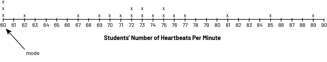 image The Number line is titled "Students’ Number of Heartbeats Per Minute". It is graduated from 60 to 90. With an arrow, the word "mode" points to the number 60. The numbers that have no X's are: 61, 63, 64, 65, 66, 68, 78, 79, 80, 82, 83, 84, 86, 87, 88, and 90. The numbers 62, 67, 69, 70, 71, 74, 76, 77, 81, 85 and 89 have an X. The numbers 72, 73 and 64 have two X's. The number 60 has three X's.
Mean
In mathematics, mean corresponds to the value resulting from an equitable division. For example, if five friends have raised $5, $7, $7, $8, and $8, respectively, and they pool those amounts to share equally, each will receive $7. The mean of the amounts collected is therefore equal to $7. In more advanced mathematics, this mean is called the arithmetic mean. Other means exist (for example, geometric mean, harmonic mean), but they are not under study in the Junior Division. Teachers should emphasize understanding the concept of the mean over memorizing the usual algorithm (sum of data divided by number of data). To do this, teachers should provide students with activities that use the equal-share model or the balance model between the sum of the shortages (differences between the average and the data that are below the average) and the sum of the surpluses (differences between the mean and data that is greater than the mean). Otherwise, students gain only a limited understanding of the concept of mean.
Equal Share
The examples below demonstrate different situations that use the equal share model and help develop a good understanding of the concept of a mean. The equal share model can be used to determine a mean without having to use the standard algorithm.
Example 1
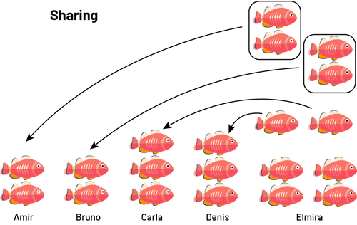
Amir, Bruno, Carla, Denis and Elmira went fishing and caught 2, 2, 3, 3 and 10 fish respectively. Determine the average number of fish caught.
To determine the mean of the number of fish caught, students can determine how many fish each person would have if the fish were evenly distributed. They can first illustrate the initial situation as follows.
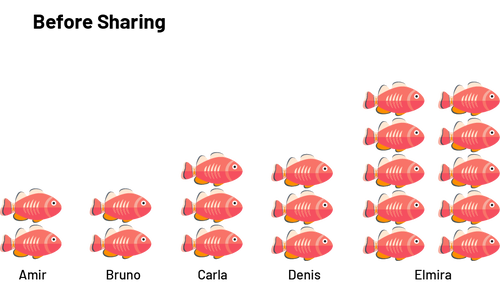 image Title of the example : Before sharing.Images of goldfish are stacked above the names of 5 students. Amir has two fish, Bruno has two fish, Carla has 3 fish, Denis has 3 fish, and Elmira has 10 fish.
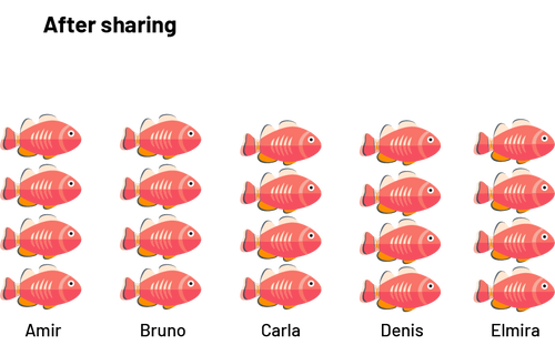
Then the students proceed to the equal sharing: Elmira gives two fish to Amir, two fish to Bruno, one fish to Carla and one fish to Denis.
After sharing, each person has four fish, so we can conclude that on average each individual caught four fish.
In order to deepen the concept of mean, it is important to give students the opportunity to reverse the process by asking them to create a set of data with a given mean. This reinforces the concept of mean as the result of equal sharing.
Example 2
Six students in a class determined that they had, on average, five pens each. What might be a possible distribution of pens among these six students?
Since the six students have an average of five pens each, each student would have five pens after the equal share.
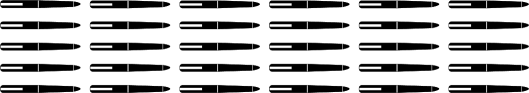
This gives a total of 30 pens (6 × 5).The six students can then divide the 30 pens among themselves as they see fit. Regardless of the division chosen, the mean value of 5 (average of five pens per student) will be maintained. Here is an example of a possible division:
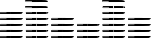
We can verify that there are still a total of 30 pens.
One can use the equal share model to develop an understanding of the usual algorithm as illustrated in the example. The model indeed makes sense of the usual algorithm, as it demonstrates the idea of grouping pens and then sharing them among friends (the sum of the values divided by the number of values).
Example 3
Five students have been asked to fundraise. If each student raises an average of $25, the group wins tickets to a hockey game. On Monday, four of the five students meet and find that they have raised $29, $21, $31 and $13. What is the minimum amount that Suzie, the fifth student, must raise for the group to win the hockey tickets?
Students who have only learned to use the standard algorithm for determining the average are often unable to answer such questions. It is a recipe that they are unable to adapt to their circumstances because they do not understand it. Students who have developed an understanding of the concept of averaging as sharing are better able to solve this problem. Here is an exchange that the four students might have to determine how much money Suzie should have collected.
Student 1 - We must obtain a mean of $25, which means that if we divided the money equally between us, we would each have $25. I collected $29, so I can share $4 with you.
Student 2 – I only got $21; so I'm missing $4.
Student 3 - I have an extra $6 because I collected $31.
Student 4 - I'm sorry. I was sick this weekend and only raised $13. I am $12 short.
Student 1 - Let's use the idea of sharing to help us figure out how much money Suzie will need to have collected to achieve an average of $25.
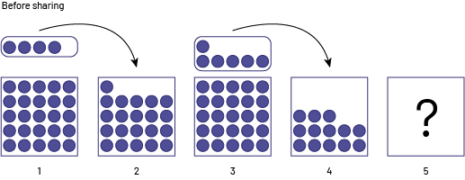 image Under the title "Before Sharing", five boxes are lined up side by side. The first box contains 25 chips. Above it, a set of 4 chips is linked to the second box by an arrow. The second box contains 21 chips. The third box contains 25 chips, and above it, a set of 6 chips points to the fourth box with an arrow. The fourth box contains 13 chips. The fifth box contains no chips, but has a question mark.
As a result of the sharing, the first three students now have $25 and the fourth student is $6 short of $25. Suzie must bring the missing $6 in addition to her $25. She must have $31.
Balance Between the Sum of the Surpluses and the Sum of the Shortages
Teachers can also help students develop an understanding of the concept of mean by presenting them with situations that involve the surplus/shortage balance model. This model, which is a variation of the equal-share model, is perhaps less familiar. It is based on the idea that if, for example, a group of students has an average number of tokens, some students might have fewer than the mean while others might have more. However, the total of what the students have fewer of must equal the total of what the students have more of. The two examples below illustrate this idea.
Example 1
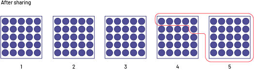
Five students each have four tokens. Annie gives one token to Carl and one token to Daniel. Bahéya gives one token to Carl and two tokens to Eva.
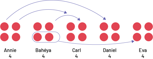
The mean is still four tokens per person. However, compared to the average, Annie has a shortage of two tokens, Bahéya has a shortage of three tokens, Carl has a surplus of two tokens, Daniel has a surplus of one token, and Eva has a surplus of two tokens. Therefore, compared to the mean, the sum of the shortages is five tokens (2 + 3), and the sum of the surpluses is five tokens (2 + 1 + 2). We can see that the sum of the shortages equals the sum of the surpluses.
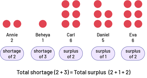 image Five sets of red chips lined up side by side have the following names respectively: Annie, Bahéya, Carl, Daniel, Eva. The first set contains two chips and indicates a lack of two. The second set contains one chip and indicates a lack of three. The third set contains 6 chips and indicates a surplus of two. The fourth set contains five chips and indicates a surplus of one. And the fifth set contains 6 chips and indicates a surplus of two. Below the sets appears the following equation: sum of the lacks opening parenthesis two plus three closing parenthesis equals sum of the surpluses opening parenthesis two plus one plus two closing parenthesis.
The surplus-shortage equilibrium model can be used to solve various problems involving the mean. For example, the situation presented in Example 3 of the “Equal Share” section above and solved using the sharing model can just as easily be solved using the surplus-shortage equilibrium model.
Example 2
Five students have been asked to fundraise. If each student raises an average of $25, the group wins tickets to a hockey game. On Monday, four of the five students meet and find that they have raised $29, $21, $31, and $13. What is the minimum amount that Suzie, the fifth student, must raise for the group to win the hockey tickets?
Each amount of money is first examined against the average of $25 and the surplus or shortfall is determined.
29: $4 surplus
21: $4 shortage
31: $6 surplus
13: $12 shortage
The sum of the surpluses and the sum of the shortages are then determined.

These two amounts are not equal, so to balance them out, we need an extra $6 ($16 - $10), so Suzie must have collected $25 + $6, or $31.
Once students have developed a good understanding of the concept of mean, they are able to:
- determine the mean of a data set and understand the relationship between the data and the mean;
- create a set of data that corresponds to a particular mean and understand that the same mean can come from more than one set of data;
- determine a missing data item from a set of data to obtain a particular mean and understand the effect on the mean of adding new data.
Only when this understanding is achieved should they be introduced to the usual algorithm for calculating the mean, which is:

Note that focusing on conceptual understanding of the mean avoids some of the following conceptual errors that were identified by Konold and Higgins (2003, pp. 203-204):
- some students confuse the mean with the mode, in other words, they associate it with the most frequent value;
- some students associate the mean only with an algorithm, which makes it difficult for them to create a data set that corresponds to a particular mean;
- some students mistake the mean for the median, that is, they associate it with the value in the center of the set of data.
Even with a good understanding of statistical measures, it is not always easy to choose the best one for a given situation in a decision-making context, so in the Junior Division it is best to stick to simple situations.
Example
Matthew wants to negotiate with his parents for an increase in the amount of weekly allowance he receives. Knowing that he cannot simply ask for an increase without good reason, he decides to survey his fellow students to find out how much allowance they receive each week. He organizes the data he has collected on a line plot.
 image The number line shows weekly amounts of pocket money in dollars, with "X's". At zero, there are four X's. At one, there is one "X". At one and a half, there are two X's. At two, there are two X's. At two and a half, there is an "X". At three, there is an "X". At three and a half, there are four X's. At four, there are five X's. At four and a half, there are four "X's". At five, there are five X's. At five and a half, there are two "X's". At six, there are four "X's". At six and a half, there are no "X's". At seven, there is one "X". At seven and a half, there is no "X". At eight, there is an "X". At eight and a half, nine and nine and a half, there is no "X". And at ten, there are six X's.
Matthew then analyzes this data to choose a value on which to base his arguments for an increase in allowance. Noting that $10 is the most common value, he goes to his father and explains that, according to his survey, more of his peers receive $10 in spending money than any other amount.
His father finds this amount rather high and asks to see the data set. After reviewing it, he explains to Matthew that because of the distribution of the data, mode is not the best measure to represent the data. Then he determines that the mean of the amounts allocated is $4.66 and tells Matthew that this amount seems more appropriate.
A bit disappointed, Matthew calculates the median and finds that it is $4.50. He understands that in this situation, both the mean and the median are good measures to represent the data, but since the median is lower than the mean, he decides that it is not to his advantage to use it.
Source: translated from Guide d’enseignement efficace des mathématiques, de la 4e à la 6e année, Traitement des données et probabilité, p. 115-125.
Median
The median of a set of data is the number in the middle of this ordered set such that there is an equal amount data values on either side. In the case of an even number of data, the median is the number that is halfway (average) between the two middle numbers. In such cases, the median may be a number that is not part of the set of data.
Example 1
The data below was recorded during a long jump competition.
1.04 m; 1.06 m; 1.12 m; 1.13 m; 1.16 m; 1.19 m; 1.22 m; 1.28 m; 1.36 m
The nine data values are in ascending order. The median of this data set is the fifth data value, which is 1.16 m. Notice that there are four data values on each side of the median.
Example 2
The stem-and-leaf plot below shows 22 pieces of data placed in ascending order. Two pieces of data are in the middle, the 11th and 12th pieces of data. Note that there is an equal amount of data values (ten) on either side of these two middle numbers. Since the 11th and 12th values are both 72 heartbeats per minute, the median will also be 72 heartbeats per minute.
| Number of Heartbeats per Minute of Students in the Class | |
|---|---|
| 6 | 3 5 5 8 9 |
| 7 | 1 1 2 2 2 2 2 4 5 7 7 |
| 8 | 2 3 6 |
| 9 | 1 2 |
| 10 | 8 |
Example 3
At a fundraiser for their sports team, 10 students sold boxes of chocolate. Here are the numbers of boxes sold:
15, 12, 11, 10, 10, 8, 7, 6, 5, 5
The data set of 10 data values has been arranged in descending order. The 5th and 6th values are in the centre of this set. These two data values, 10 and 8, are different. The median is 9, since 9 is halfway between 8 and 10. Despite the fact that this median is not part of the data set, we can see that there are the same number of data values (five) on either side of it.
Example 4
Here is the data for the maximum daily temperature, in degrees Celsius, in a city in August.
| Maximum Temperatures in August (°C) | ||||||
|---|---|---|---|---|---|---|
| 17 | 20 | 19 | 25 | 27 | 28 | 30 |
| 29 | 27 | 22 | 21 | 20 | 25 | 29 |
| 32 | 33 | 33 | 27 | 24 | 17 | 21 |
| 26 | 25 | 27 | 24 | 21 | 23 | 25 |
| 16 | 18 | 19 | ||||
To determine the median, students need to first put the values in ascending or descending order. They can use an intermediate stem-and-leaf plot as follows. Students may first identify the stems that are needed and arrange them in order.
| 1 | 7 | 9 | 7 | 6 | 8 | 9 | ||||||||||
| 2 | 0 | 5 | 7 | 8 | 9 | 7 | 2 | 1 | 0 | 5 | 9 | 7 | 4 | 1 | 3 | 5 |
| 3 | 0 | 2 | 3 | 3 |
Students can then place the leaves in each row in ascending order and get the following graph.
| 1 | 6 | 7 | 7 | 8 | 9 | 9 | |||||||||||||||
| 2 | 0 | 0 | 1 | 1 | 1 | 2 | 3 | 4 | 4 | 5 | 5 | 5 | 5 | 6 | 7 | 7 | 7 | 7 | 8 | 9 | 9 |
| 3 | 0 | 2 | 3 | 3 |
To help students determine the median, teachers may suggest that they write the numbers in order on a strip of paper and fold it as follows.

Using the paper strip helps students develop a better understanding of the concept of median, since by folding the strip in half, the numbers are paired (first to last, second to second to last, and so on) and only one piece of data is in the middle. It is then easy to see that the median of the data is 25°C.
Example 5
The graph below shows the maximum daily temperatures for a city during the month of June, in degrees Celsius.
| Daily Maximum Temperatures in June (°C) | |||||||||||||||||||
|---|---|---|---|---|---|---|---|---|---|---|---|---|---|---|---|---|---|---|---|
| 1 | 2 | 4 | 6 | 6 | 7 | 8 | 9 | ||||||||||||
| 2 | 0 | 0 | 1 | 1 | 1 | 1 | 3 | 4 | 5 | 5 | 6 | 6 | 7 | 7 | 8 | 8 | 9 | 9 | 9 |
| 3 | 0 | 2 | 3 | 3 | |||||||||||||||
Have students copy the numbers from the stem-and-leaf plot onto a strip of paper. Next have the students fold the paper in half. In this case the fold should be between the two numbers in the middle, 24 and 25. Students can use their knowledge of decimal numbers to determine that it is the number 24.5 that is halfway between 24 and 25. The median of this data set is therefore 24.5°C.

The median is an important statistical measure that is commonly used in many situations. Because it indicates the value at the centre of an ordered set of data, it is possible to place all other values in relation to the median. For example, in the example of the long jump competition (Example 1), the student who successfully jumped 1.28 m knows that the length of this jump is greater than the median of 1.16 m and, therefore, greater than the length of most of the other jumps.
Before using the median to make decisions, however, it is important to consider the range of the data because the median does not take into account extreme values. In the example of the sale of boxes of chocolate (Example 3), we are trying to estimate the number of boxes that were sold. We know that the median number of boxes sold is 9 and that the data range is from 5 to 15 boxes. Therefore, the range of the data is small, and the median, 9, is almost halfway between the maximum and the minimum value. Therefore, it can be assumed that each student sold about 9 boxes and concluded that the 10 students sold about 90 boxes.
Now imagine a situation with the same data, however the largest number of boxes sold is 75, not 15. The median is still 9 boxes, but the range is very large. Also, the median is not at all halfway between the maximum and minimum values, so one could not assume that each student sold about 9 boxes, as in the previous situation, and conclude that the 10 students sold about 90 boxes in total.
Teachers can also help students deepen their understanding of the concept of median by modifying some of the situations they have already studied, as shown in the following example.
Example 6
Let's alter Example 3 as follows:
At a fundraiser for their sports team, 10 students sold boxes of chocolate. Here are the numbers of boxes sold.
15, 12, 11, 10, 10, 8, 7, 6, 5, 5
However, three students have not yet reported their number of boxes sold. If the goal was to obtain a median number of eight boxes sold, what data set corresponding to the sales of the 13 students could meet this goal?
Here are two examples of possible answers.
15, 12, 11, 10, 10, 8, 8, 7, 7, 6, 5, 5, 4
15, 12, 11, 10, 10, 9, 8, 7, 6, 5, 5, 4, 3
If we add as a condition that the mode of the data set also corresponds to eight boxes, students could give the following answer.
15, 12, 11, 10, 10, 8, 8, 8, 7, 6, 5, 5, 4
Source: translated from Guide d’enseignement efficace des mathématiques, de la 4e à la 6e année, Traitement des données et probabilité, p. 111-115.